
Logs and correlation guide
Everything past the quick start for vertical wells: tuning tracks, picking and pinching out tops, sections, zone stats, curve QC, maps and scanned logs.
1. Tracks and curves
Click a curve's scale in a track header to edit that curve in every well: display name, which curve, color, line style and width, left and right scale, log scale, wrap, and a fill (solid, or colored by value). A track's ⚙ opens the full track editor along the bottom, with every curve in the track, its width and name; Apply keeps the changes, Cancel or Esc puts them back.
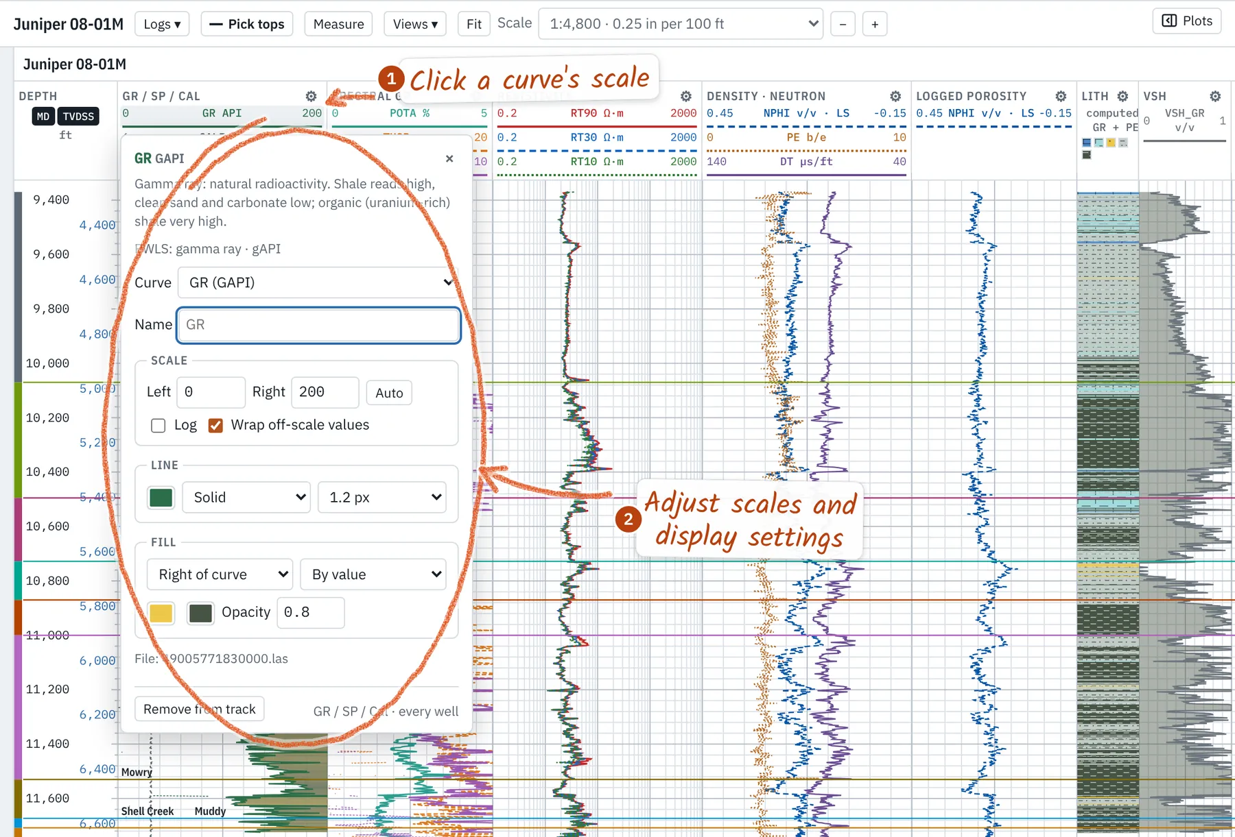
- Logs ▾ beside the well name lists every curve by what it measures; a checkbox shows or hides it. The ▸ before a well in the Wells list does the same.
- Several curves of one kind (two GRs, two deep resistivities): open-hole beats cased-hole and the longest run wins. Pick another, or overlay them all, in the well's ⚙.
- + track adds a track; show empty lists tracks with no data in the open wells. Save as my defaults in the track editor keeps the set for new projects.
- Lithology is computed from GR and PE cutoffs; its ⚙ edits the cutoffs, colors and FGDC-style patterns. Hover it for the class and the values behind it.
- Unknown mnemonics are asked about once, with a guess from the unit, range and description, and remembered for that service company or every file (Curve QC → Curve mappings…).
2. Well headers and surveys
Manage wells renames wells, fills operator, field, county, state, location and elevations for several at once, merges selected wells or splits a merged well back into its files. Hover a well name for its header. LAS files with the same API merge into one well; a sidetrack code splits them. State and county fill from the API number when a file leaves them blank.
A well's ⚙ → Load survey… reads CSV, Excel, text reports or WITSML. A review shows the column mapping, depth unit, north reference (grid with convergence, or magnetic with declination, converted to true), the tie-in and every rejected row with its reason. Loading over an existing survey runs a dry run first: append, merge or replace, with counts. TVD is by minimum curvature.
3. Picking tops
Pick tops or T opens the pick bar. 1–9 choose a top; typed names separated by commas start several, top to bottom, and auto-next moves to the next missing top after each pick. The bar lists the wells still missing the top, with an MD box for an exact depth. Picks snap to a round depth about a pixel apart, so a zoomed-in core picks to the centimeter.
- Drag a top line to move it; ↑/↓ nudge the last pick (Shift: ×10).
- [ and ] step to the previous or next well in the Logs tab, keeping the top.
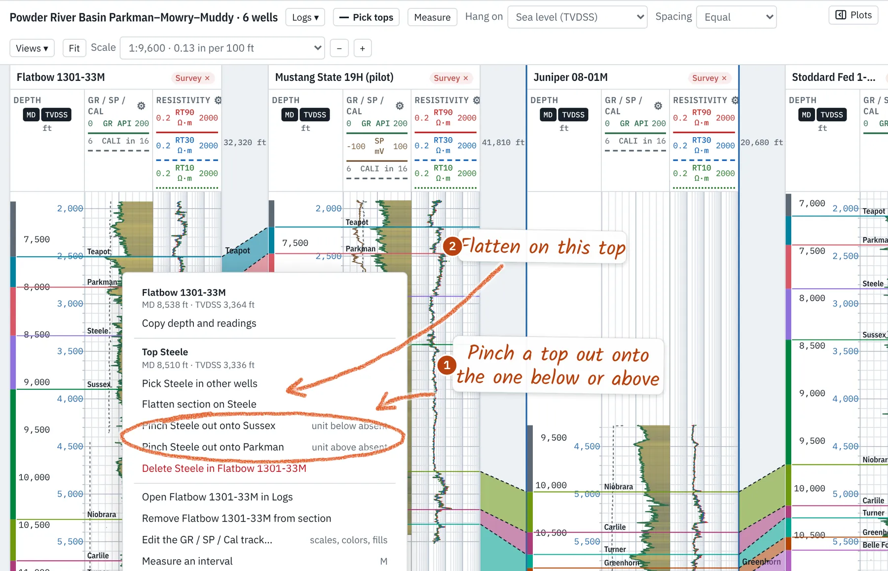
- Right-click a top → Pick … in other wells, or Flatten section on ….
- The Tops panel sets each top's color and takes typed MDs. The status bar warns when tops cross between wells or are missing.
4. Pinch-outs and absent units
Right-click a top line → Pinch … out onto the top below or above. Right-click between two tops to put the active top there, or to mark a unit the other wells have as absent here. A pinched top rides on its neighbor (dashed, marked ⋀), and the section draws the missing unit as a wedge closing midway between wells. Un-pinch undoes it.
5. Cross sections
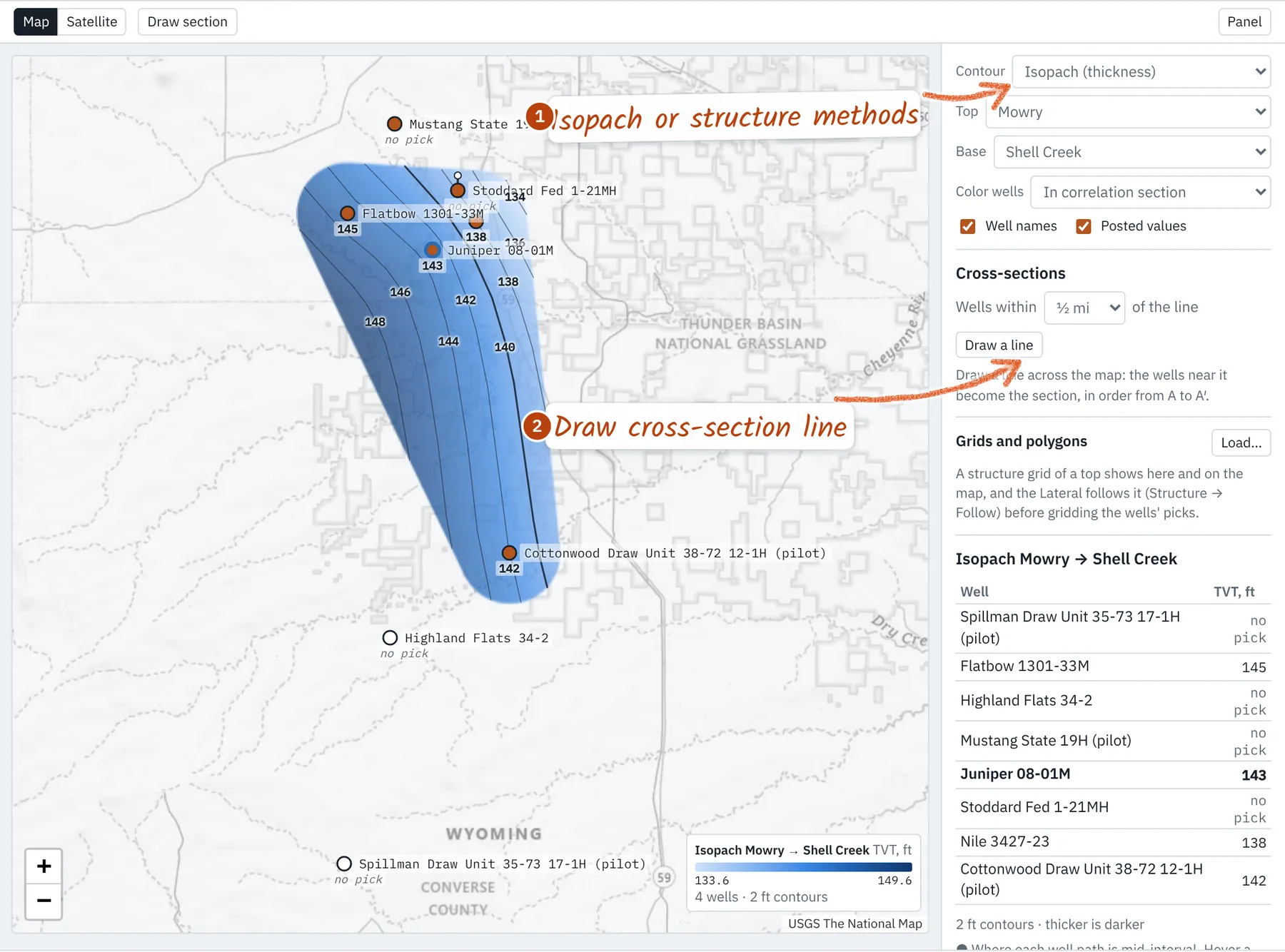
Hang on measured depth, ground level, sea level (TVDSS) or a flattened top. Spacing is equal, or by distance (labeled). Order follows the Wells list: drag rows, or on the Map tab Draw a line and the wells within a chosen distance become the section, in order from A to A′. Deviated and horizontal wells use TVD from their survey; the depth track always labels real MD and TVDSS.
- Views ▾ saves the section, hang, tracks, scale and depth under a name, and brings it back.
- Scale is a print ratio; Fit fits the window; Ctrl/⌘ + wheel zooms freely. Logs and Correlation keep their own zoom.
- Measure (M) drags out an interval: MD thickness, true vertical thickness and depths at top and base.
6. Point data
Core measurements, pressures, XRD and other values at depth load from CSV or Excel: well (or API), MD, then a column per measurement, units in the header such as k (mD). They plot as markers on any track. Labeled depths (perforations, shows; one depth, or a top and base) land in one track with a lane and color per class; Split in the Point data panel gives each class its own track. Depths can be MD or TVD (converted through the survey).
7. Interpretation
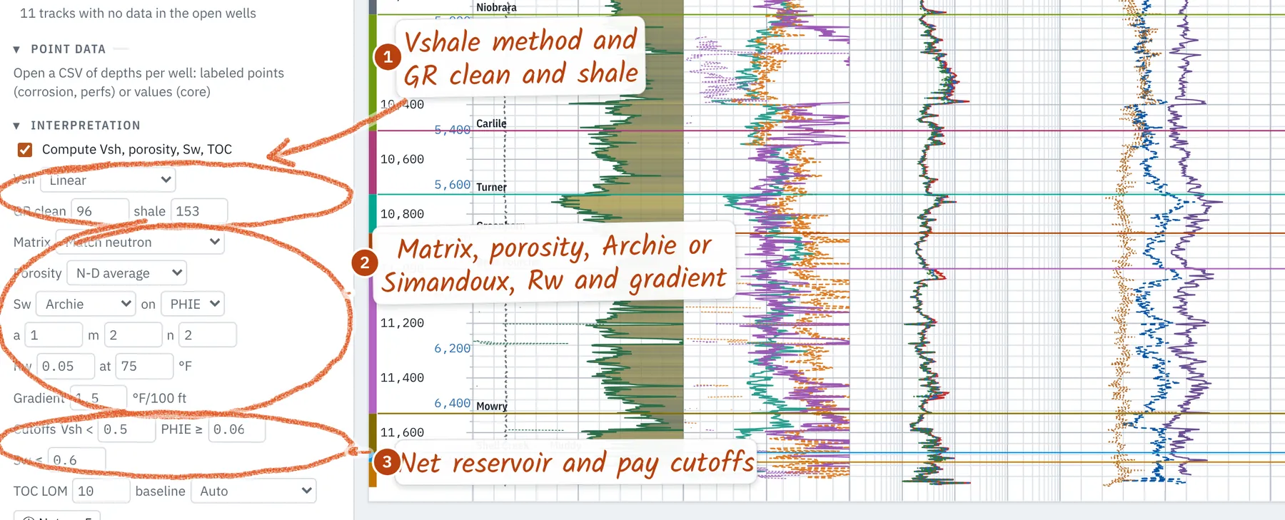
The Interpretation panel sets the quick-look petrophysics: Vshale (linear, Larionov, Clavier) with clean and shale GR, neutron-density porosity, Archie or Simandoux water saturation with Rw corrected for temperature, Passey ΔlogR TOC, bad-hole flags, and net reservoir and pay cutoffs. Every parameter is saved with the project; the equations are in Methods.
8. Zone stats and plots
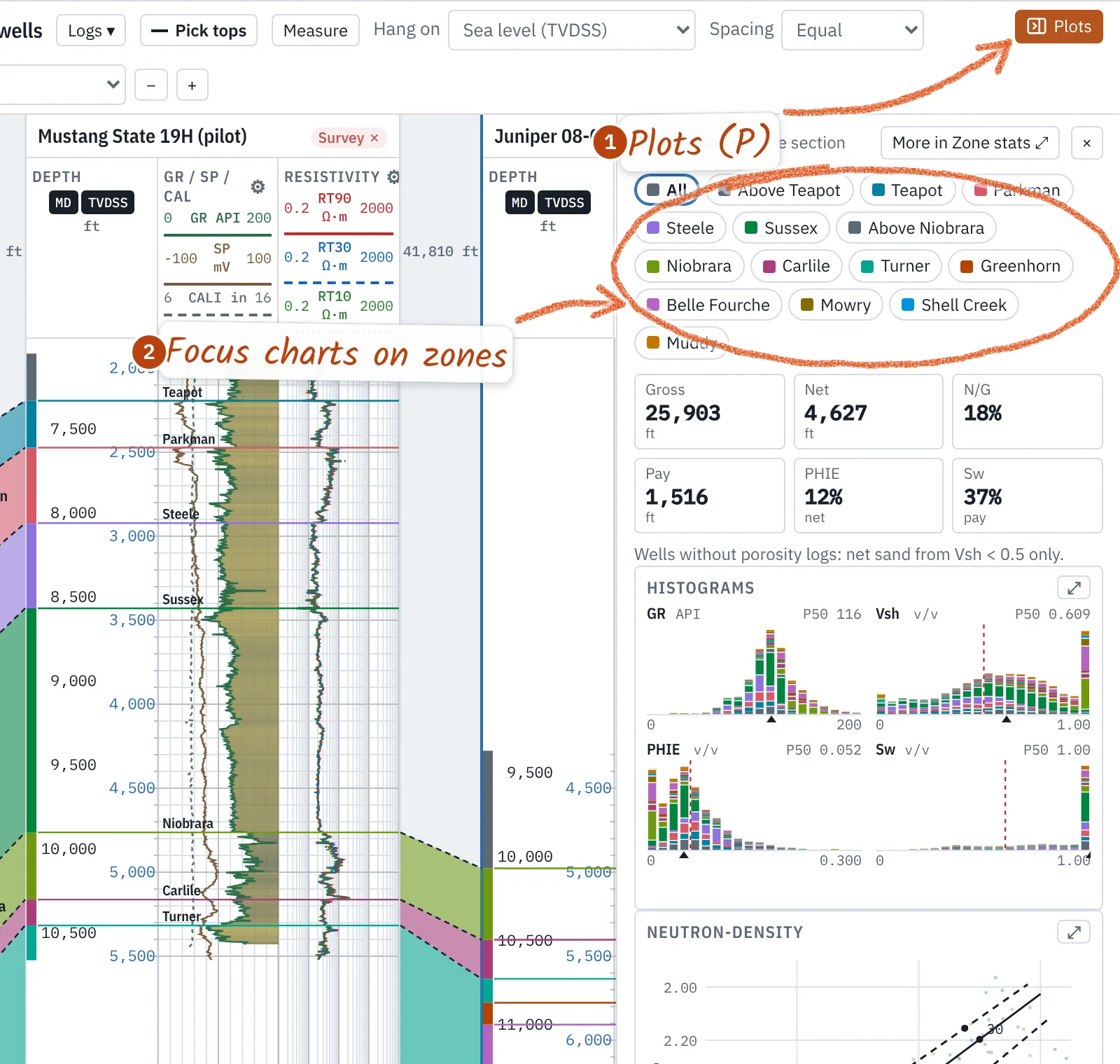
Zone stats gives distributions by zone and well, crossplots (neutron-density with lithology lines, Pickett with Sw lines, PE-density, or any two curves) colored by zone, GR band or well, histograms, and a summary table: gross, net, net-to-gross, pay, average porosity and Sw, porosity-feet and hydrocarbon-feet, in true vertical thickness for deviated wells. Click a zone to hide it; hide bad hole drops washouts. Every chart has a PNG button.
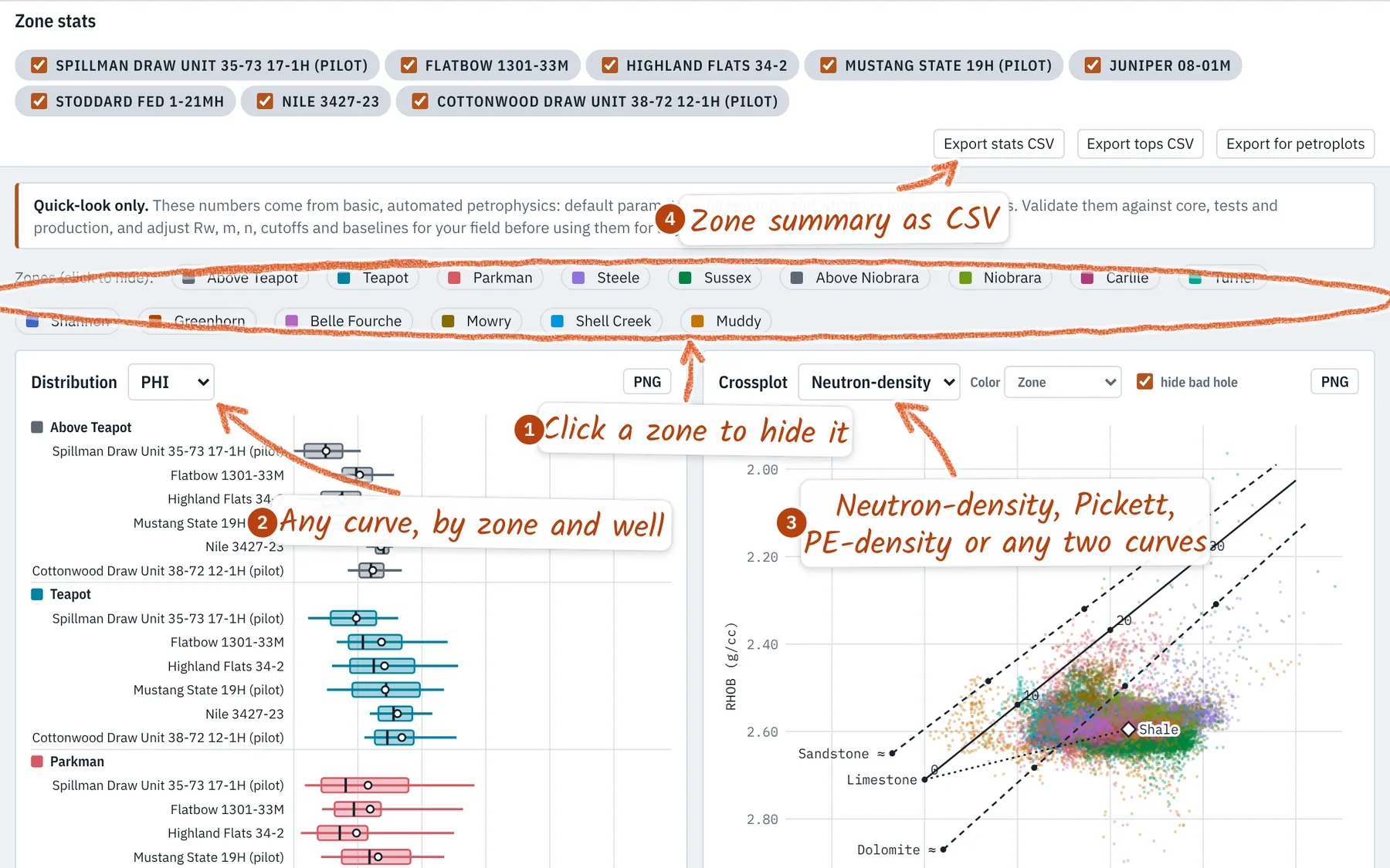
Plots (P) opens the key charts beside the logs or section for the wells on screen; pick a zone to focus them, or ⤢ for the full charts.
9. Curve QC
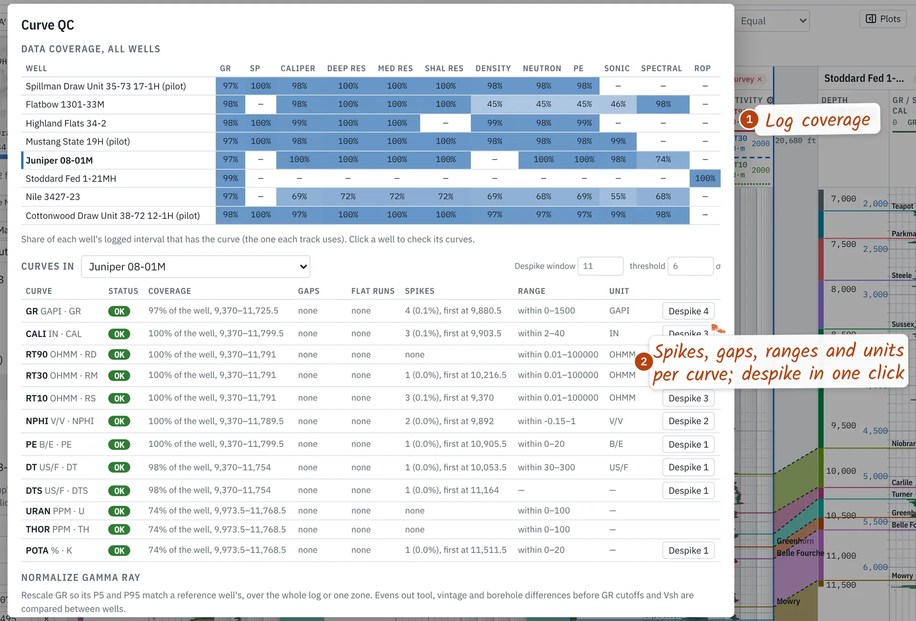
Curve QC in the Wells panel shows which wells have which logs, then checks each curve of a well for coverage, gaps, flat runs, spikes, physical range and units. Despike replaces spikes with a rolling median; Normalize GR rescales a well's P5–P95 onto a reference well's, over the whole log or one zone. Edits are saved with the project and undo with Ctrl+Z.
10. Maps
The Map tab contours an isopach between two tops or a structure map on one, from every well's picks, with a thin-plate spline inside the wells' hull. Each well posts its value; hover for the gridded value. Contours every sets the interval (20 by default; Auto picks about ten lines). Color wells fills well dots by a property. Structure grids from other software (ZMAP+, CPS-3, XYZ) and polygons (GeoJSON or x y lists) load like any file; their coordinate system is found from the open wells, and their values are fitted to the picks to tell depth from elevation.
11. PDF and TIFF logs
The PDF / raster tab lines up to eight scanned or vector logs side by side. Each new file opens on a review of its pages: crop by blank margins (default), the ruled plot frame, or nothing; drag the handles to crop, or drag on the page to draw a crop or cut a page break. Where the PDF has text, the depth column is found and fitted page by page. Scans without text take two clicks on ruled depth lines (type each MD); later pages follow at that scale.
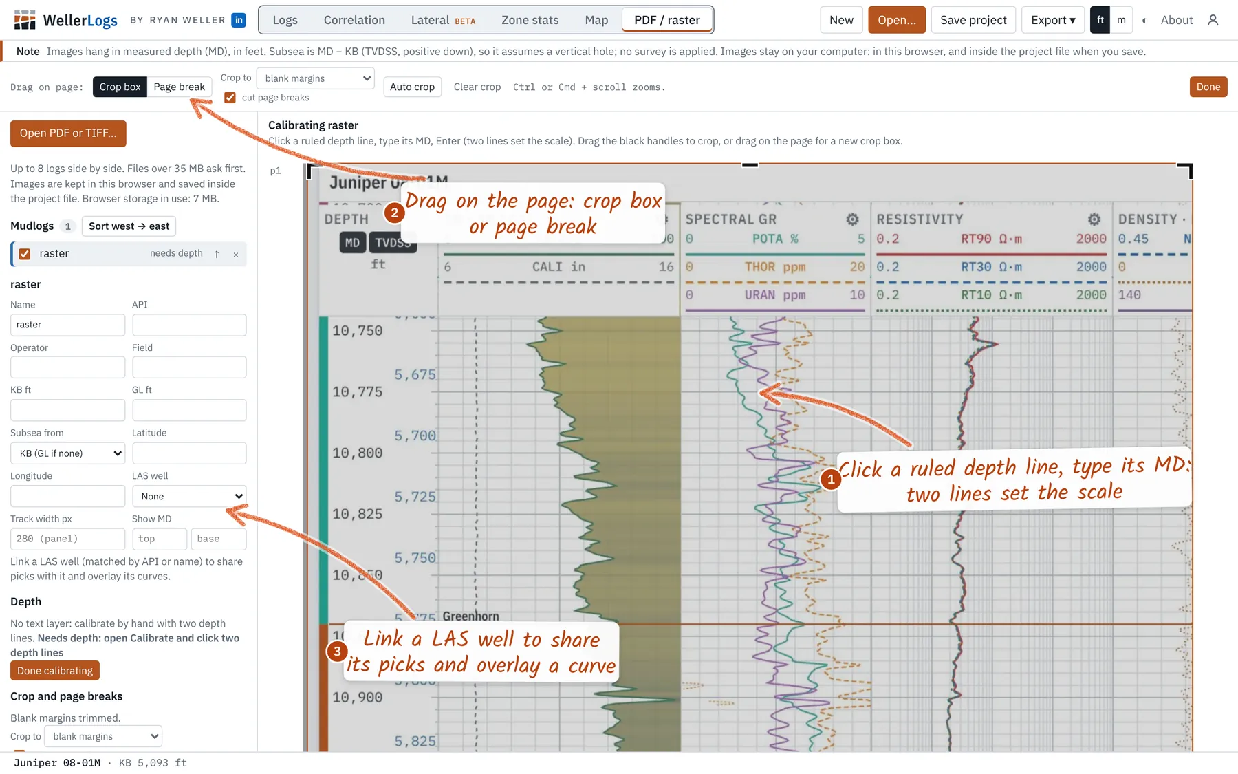
- Hang on MD, subsea (MD − KB) or a pick; Sort west → east orders by longitude.
- Link a LAS well (matched by API or name) to share its picks and draw one of its curves over the scan.
- Drag a log's right edge to set its width; double-click for its printed shape. Images are kept in the browser and saved in the project.
12. Exports and printing
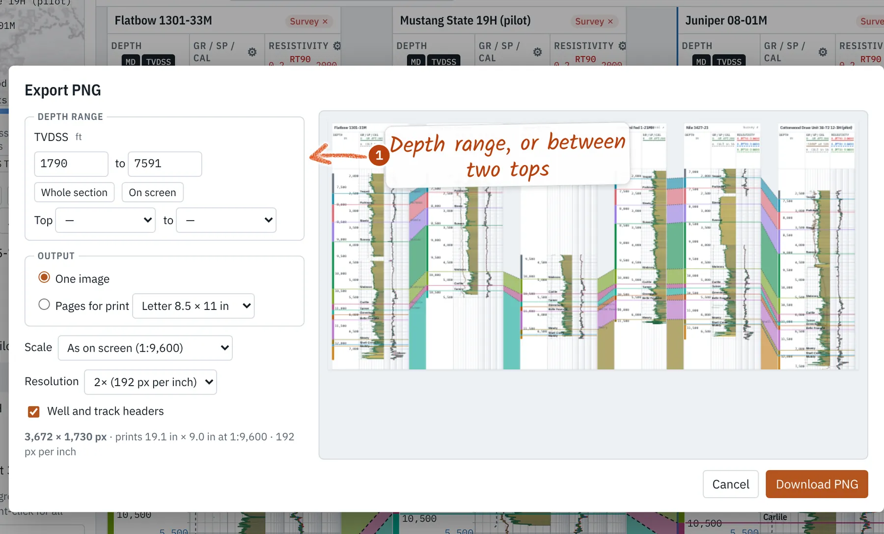
Export → PNG image or print pages (Ctrl+E) sets the depth range or the interval between two tops, one image or pages to print at a true scale, resolution, headers and a white background, with a preview. Export also writes the selected or all wells as LAS 2.0 (shifts, despiking and computed curves included), tops and zone stats as CSV, and a full project bundle. Zone stats also exports curves in petroplots names for publication figures.
13. Mouse and hot keys
- T Pick tops · 1–9 choose a top
- ↑ ↓ Nudge the last pick (Shift: ×10)
- [ ] Previous or next well
- M Measure · P Plots
- Ctrl+E Export PNG · Ctrl+S Save
- Ctrl+Z Undo · Esc Close or stop
- Ctrl/⌘ + wheel: zoom freely
- Right-click a log or top: options there
14. Additional features
- Robust LAS reading: LAS 1.2, 2.0 and 3.0, wrapped data, odd nulls, swapped header fields, bottom-up logs; a file that won't load says why.
- JSON Well Log Format and WITSML logs, trajectories and formation markers open like LAS.
- Cores and geotechnical logs: scales down to 1:1, cm and mm depths, Scale → Custom… for a typed scale or depth range.
- MWD / LWD: sensor-to-bit offsets listed per tool and applied in one click; azimuthal GR and inclination tracks.
- Cased hole: cement bond, ultrasonic cement, casing and temperature tracks where the curves exist.
Equations, defaults and limits: Methods.